libigl_Martin/tutorial/readme.md

title: libigl Tutorial author: Alec Jacobson, Daniele Pannozo and others date: 20 June 2014 css: style.css html header:

Introduction

Libigl is an open source C++ library for geometry processing research and development. Dropping the heavy data structures of tradition geometry libraries, libigl is a simple header-only library of encapsulated functions. % This combines the rapid prototyping familiar to \textsc{Matlab} or \textsc{Python} programmers with the performance and versatility of C++. % The tutorial is a self-contained, hands-on introduction to \libigl. % Via live coding and interactive examples, we demonstrate how to accomplish various common geometry processing tasks such as computation of differential quantities and operators, real-time deformation, global parametrization, numerical optimization and mesh repair. % Accompanying lecture notes contain further details and cross-platform example applications for each topic. \end{abstract}

Index

• 100_FileIO: Example of reading/writing mesh files
• 101_Serialization: Example of using the XML serialization framework
• 102_DrawMesh: Example of plotting a mesh
• 202 Gaussian Curvature
• 203 Curvature Directions
• 204 Gradient

Compilation Instructions

All examples depends on glfw, glew and anttweakbar. A copy of the sourcecode of each library is provided together with libigl and they can be precompiled using:

Alec: Is this just compiling the dependencies? Then perhaps rename compile_dependencies_*

sh compile_macosx.sh (MACOSX)
sh compile_linux.sh (LINUX)
compile_windows.bat (Visual Studio 2012)

Every example can be compiled by using the cmake file provided in its folder. On Linux and MacOSX, you can use the provided bash script:

sh ../compile_example.sh

(Optional: compilation with libigl as static library)

By default, libigl is a headers only library, thus it does not require compilation. However, one can precompile libigl as a statically linked library. See ../README.md in the main directory for compilations instructions to produce libigl.a and other libraries. Once compiled, these examples can be compiled using the CMAKE flag -DLIBIGL_USE_STATIC_LIBRARY=ON:

../compile_example.sh -DLIBIGL_USE_STATIC_LIBRARY=ON

Chapter 2: Discrete Geometric Quantities and Operators

This chapter illustrates a few discrete quantities that libigl can compute on a mesh. This also provides an introduction to basic drawing and coloring routines in our example viewer. Finally, we construct popular discrete differential geometry operators.

Gaussian Curvature

Gaussian curvature on a continuous surface is defined as the product of the principal curvatures:

$k_G = k_1 k_2.$

As an intrinsic measure, it depends on the metric and not the surface's embedding.

Intuitively, Gaussian curvature tells how locally spherical or elliptic the surface is ( $k_G>0$ ), how locally saddle-shaped or hyperbolic the surface is ( $k_G<0$ ), or how locally cylindrical or parabolic ( $k_G=0$ ) the surface is.

In the discrete setting, one definition for a ``discrete Gaussian curvature'' on a triangle mesh is via a vertex's angular deficit:

$k_G(vi) = 2π - \sum\limits{j\in N(i)}θ_{ij},$

where $N(i)$ are the triangles incident on vertex $i$ and $θ_{ij}$ is the angle at vertex $i$ in triangle $j$ [][#meyer_2003].

Just like the continuous analog, our discrete Gaussian curvature reveals elliptic, hyperbolic and parabolic vertices on the domain.

Curvature Directions

The two principal curvatures $(k_1,k_2)$ at a point on a surface measure how much the surface bends in different directions. The directions of maximum and minimum (signed) bending are call principal directions and are always orthogonal.

Mean curvature is defined simply as the average of principal curvatures:

$H = \frac{1}{2}(k_1 + k_2).$

One way to extract mean curvature is by examining the Laplace-Beltrami operator applied to the surface positions. The result is a so-called mean-curvature normal:

$-\Delta \mathbf{x} = H \mathbf{n}.$

It is easy to compute this on a discrete triangle mesh in libigl using the cotangent Laplace-Beltrami operator [][#meyer_2003].

#include <igl/cotmatrix.h>
#include <igl/massmatrix.h>
#include <igl/invert_diag.h>
...
MatrixXd HN;
SparseMatrix<double> L,M,Minv;
igl::cotmatrix(V,F,L);
igl::massmatrix(V,F,igl::MASSMATRIX_VORONOI,M);
igl::invert_diag(M,Minv);
HN = -Minv*(L*V);
H = (HN.rowwise().squaredNorm()).array().sqrt();

Combined with the angle defect definition of discrete Gaussian curvature, one can define principal curvatures and use least squares fitting to find directions [][#meyer_2003].

Alternatively, a robust method for determining principal curvatures is via quadric fitting [][#pannozo_2010]. In the neighborhood around every vertex, a best-fit quadric is found and principal curvature values and directions are sampled from this quadric. With these in tow, one can compute mean curvature and Gaussian curvature as sums and products respectively.

This is an example of syntax highlighted code:

#include <foo.html>
int main(int argc, char * argv[])
{
  return 0;
}

Gradient

Scalar functions on a surface can be discretized as a piecewise linear function with values defined at each mesh vertex:

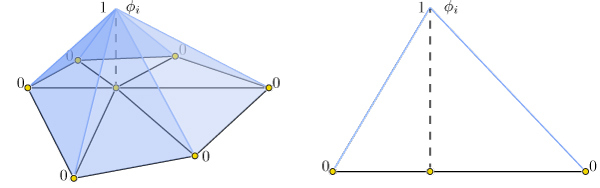
$f(\mathbf{x}) \approx \sum\limits_{i=0}^n \phi_i(\mathbf{x})\, f_i,$

where $\phi_i$ is a piecewise linear hat function defined by the mesh so that for each triangle $\phi_i$ is the linear function which is one only at vertex $i$ and zero at the other corners.

Thus gradients of such piecewise linear functions are simply sums of gradients of the hat functions:

$\nabla f(\mathbf{x}) \approx \nabla \sum\limits_{i=0}^n \nabla \phi_i(\mathbf{x})\, fi = \sum\limits{i=0}^n \nabla \phi_i(\mathbf{x})\, f_i.$

This reveals that the gradient is a linear function of the vector of $f_i$ values. Because $\phi_i$ are linear in each triangle their gradient are constant in each triangle. Thus our discrete gradient operator can be written as a matrix multiplication taking vertex values to triangle values:

$\nabla f \approx \mathbf{G}\,\mathbf{f},$

where $\mathbf{f}$ is $n\times 1$ and $\mathbf{G}$ is an $m\times n$ sparse matrix. This matrix $\mathbf{G}$ can be derived geometrically, e.g. [ch. 2][#jacobson_thesis_2013]. Libigl's gradMatAlec: check name function computes $\mathbf{G}$ for triangle and tetrahedral meshes:

[#meyer_2003]: Mark Meyer and Mathieu Desbrun and Peter Schröder and Alan H. Barr, "Discrete Differential-Geometry Operators for Triangulated 2-Manifolds," 2003. [#pannozo_2010]: Daniele Pannozo, Enrico Puppo, Luigi Rocca, "Efficient Multi-scale Curvature and Crease Estimation," 2010. [#jacobson_thesis_2013]: Alec Jacobson, Algorithms and Interfaces for Real-Time Deformation of 2D and 3D Shapes, 2013.