libigl_Martin/tutorial/readme.md

title: libigl Tutorial author: Alec Jacobson, Daniele Pannozo and others date: 20 June 2014 css: style.css html header:

Introduction

Libigl is an open source C++ library for geometry processing research and development. Dropping the heavy data structures of tradition geometry libraries, libigl is a simple header-only library of encapsulated functions. This combines the rapid prototyping familiar to Matlab or Python programmers with the performance and versatility of C++. The tutorial is a self-contained, hands-on introduction to libigl. Via live coding and interactive examples, we demonstrate how to accomplish various common geometry processing tasks such as computation of differential quantities and operators, real-time deformation, global parametrization, numerical optimization and mesh repair. Each section of these lecture notes links to a cross-platform example application.

Table of Contents

• [Chapter 1: Introduction to libigl]

• Chapter 2: Discrete Geometric Quantities and Operators

  • 201 Normals
    • Per-face
    • Per-vertex
    • Per-corner
  • 202 Gaussian Curvature
  • 203 Curvature Directions
  • 204 Gradient
  • 204 Laplacian
    • Mass matrix
    • Alternative construction of Laplacian

• Chapter 3: Matrices and Linear Algebra

  • 301 Slice
  • 302 Sort
    • Other Matlab-style functions
  • 303 Laplace Equation
    • Quadratic energy minimization
  • 304 Linear Equality Constraints
  • 305 Quadratic Programming

• Chapter 4: Shape Deformation

  • 401 Biharmonic Deformation
  • 402 Polyharmonic Deformation
  • 403 Bounded Biharmonic Weights
  • 404 Dual Quaternion Skinning
  • 405 As-rigid-as-possible
  • 406 Fast automatic skinning transformations

Chapter 2: Discrete Geometric Quantities and Operators

This chapter illustrates a few discrete quantities that libigl can compute on a mesh. This also provides an introduction to basic drawing and coloring routines in our example viewer. Finally, we construct popular discrete differential geometry operators.

Normals

Surface normals are a basic quantity necessary for rendering a surface. There are a variety of ways to compute and store normals on a triangle mesh.

Per-face

Normals are well defined on each triangle of a mesh as the vector orthogonal to triangle's plane. These piecewise constant normals produce piecewise-flat renderings: the surface appears non-smooth and reveals its underlying discretization.

Per-vertex

Storing normals at vertices, Phong or Gouraud shading will interpolate shading inside mesh triangles to produce smooth(er) renderings. Most techniques for computing per-vertex normals take an average of incident face normals. The techniques vary with respect to their different weighting schemes. Uniform weighting is heavily biased by the discretization choice, where as area-based or angle-based weighting is more forgiving.

The typical half-edge style computation of area-based weights might look something like this:

N.setZero(V.rows(),3);
for(int i : vertices)
{
  for(face : incident_faces(i))
  {
    N.row(i) += face.area * face.normal;
  }
}
N.rowwise().normalize();

Without a half-edge data-structure it may seem at first glance that looping over incident faces---and thus constructing the per-vertex normals---would be inefficient. However, per-vertex normals may be throwing each face normal to running sums on its corner vertices:

N.setZero(V.rows(),3);
for(int f = 0; f < F.rows();f++)
{
  for(int c = 0; c < 3;c++)
  {
    N.row(F(f,c)) += area(f) * face_normal.row(f);
  }
}
N.rowwise().normalize();

Per-corner

Storing normals per-corner is an efficient an convenient way of supporting both smooth and sharp (e.g. creases and corners) rendering. This format is common to OpenGL and the .obj mesh file format. Often such normals are tuned by the mesh designer, but creases and corners can also be computed automatically. Libigl implements a simple scheme which computes corner normals as averages of normals of faces incident on the corresponding vertex which do not deviate by a specified dihedral angle (e.g. 20°).

Gaussian Curvature

Gaussian curvature on a continuous surface is defined as the product of the principal curvatures:

$k_G = k_1 k_2.$

As an intrinsic measure, it depends on the metric and not the surface's embedding.

Intuitively, Gaussian curvature tells how locally spherical or elliptic the surface is ( $k_G>0$ ), how locally saddle-shaped or hyperbolic the surface is ( $k_G<0$ ), or how locally cylindrical or parabolic ( $k_G=0$ ) the surface is.

In the discrete setting, one definition for a ``discrete Gaussian curvature'' on a triangle mesh is via a vertex's angular deficit:

$k_G(vi) = 2π - \sum\limits{j\in N(i)}θ_{ij},$

where $N(i)$ are the triangles incident on vertex $i$ and $θ_{ij}$ is the angle at vertex $i$ in triangle $j$ [][#meyer_2003].

Just like the continuous analog, our discrete Gaussian curvature reveals elliptic, hyperbolic and parabolic vertices on the domain.

Curvature Directions

The two principal curvatures $(k_1,k_2)$ at a point on a surface measure how much the surface bends in different directions. The directions of maximum and minimum (signed) bending are call principal directions and are always orthogonal.

Mean curvature is defined simply as the average of principal curvatures:

$H = \frac{1}{2}(k_1 + k_2).$

One way to extract mean curvature is by examining the Laplace-Beltrami operator applied to the surface positions. The result is a so-called mean-curvature normal:

$-\Delta \mathbf{x} = H \mathbf{n}.$

It is easy to compute this on a discrete triangle mesh in libigl using the cotangent Laplace-Beltrami operator [][#meyer_2003].

#include <igl/cotmatrix.h>
#include <igl/massmatrix.h>
#include <igl/invert_diag.h>
...
MatrixXd HN;
SparseMatrix<double> L,M,Minv;
igl::cotmatrix(V,F,L);
igl::massmatrix(V,F,igl::MASSMATRIX_TYPE_VORONOI,M);
igl::invert_diag(M,Minv);
HN = -Minv*(L*V);
H = (HN.rowwise().squaredNorm()).array().sqrt();

Combined with the angle defect definition of discrete Gaussian curvature, one can define principal curvatures and use least squares fitting to find directions [][#meyer_2003].

Alternatively, a robust method for determining principal curvatures is via quadric fitting [][#pannozo_2010]. In the neighborhood around every vertex, a best-fit quadric is found and principal curvature values and directions are sampled from this quadric. With these in tow, one can compute mean curvature and Gaussian curvature as sums and products respectively.

This is an example of syntax highlighted code:

#include <foo.html>
int main(int argc, char * argv[])
{
  return 0;
}

Gradient

Scalar functions on a surface can be discretized as a piecewise linear function with values defined at each mesh vertex:

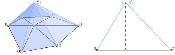
$f(\mathbf{x}) \approx \sum\limits_{i=0}^n \phi_i(\mathbf{x})\, f_i,$

where $\phi_i$ is a piecewise linear hat function defined by the mesh so that for each triangle $\phi_i$ is the linear function which is one only at vertex $i$ and zero at the other corners.

Thus gradients of such piecewise linear functions are simply sums of gradients of the hat functions:

$\nabla f(\mathbf{x}) \approx \nabla \sum\limits_{i=0}^n \nabla \phi_i(\mathbf{x})\, fi = \sum\limits{i=0}^n \nabla \phi_i(\mathbf{x})\, f_i.$

This reveals that the gradient is a linear function of the vector of $f_i$ values. Because $\phi_i$ are linear in each triangle their gradient are constant in each triangle. Thus our discrete gradient operator can be written as a matrix multiplication taking vertex values to triangle values:

$\nabla f \approx \mathbf{G}\,\mathbf{f},$

where $\mathbf{f}$ is $n\times 1$ and $\mathbf{G}$ is an $md\times n$ sparse matrix. This matrix $\mathbf{G}$ can be derived geometrically, e.g. [ch. 2][#jacobson_thesis_2013]. Libigl's gradMatAlec: check name function computes $\mathbf{G}$ for triangle and tetrahedral meshes:

Laplacian

The discrete Laplacian is an essential geometry processing tool. Many interpretations and flavors of the Laplace and Laplace-Beltrami operator exist.

In open Euclidean space, the Laplace operator is the usual divergence of gradient (or equivalently the Laplacian of a function is the trace of its Hessian):

$\Delta f = \frac{\partial^2 f}{\partial x^2} + \frac{\partial^2 f}{\partial y^2} + \frac{\partial^2 f}{\partial z^2}.$

The Laplace-Beltrami operator generalizes this to surfaces.

When considering piecewise-linear functions on a triangle mesh, a discrete Laplacian may be derived in a variety of ways. The most popular in geometry processing is the so-called ``cotangent Laplacian'' $\mathbf{L}$, arising simultaneously from FEM, DEC and applying divergence theorem to vertex one-rings. As a linear operator taking vertex values to vertex values, the Laplacian $\mathbf{L}$ is a $n\times n$ matrix with elements:

$L{ij} = \begin{cases}j \in N(i) &\cot \alpha{ij} + \cot \beta{ij},\ j \notin N(i) & 0,\ i = j & -\sum\limits{k\neq i} L_{ik}, \end{cases}$

where $N(i)$ are the vertices adjacent to (neighboring) vertex $i$, and $\alpha{ij},\beta{ij}$ are the angles opposite edge ${ij}$. This oft produced formula leads to a typical half-edge style implementation for constructing $\mathbf{L}$:

for(int i : vertices)
{
  for(int j : one_ring(i))
  {
    for(int k : triangle_on_edge(i,j))
    {
      L(i,j) = cot(angle(i,j,k));
      L(i,i) -= cot(angle(i,j,k));
    }
  }
}

Without a half-edge data-structure it may seem at first glance that looping over one-rings, and thus constructing the Laplacian would be inefficient. However, the Laplacian may be built by summing together contributions for each triangle, much in spirit with its FEM discretization of the Dirichlet energy (sum of squared gradients):

for(triangle t : triangles)
{
  for(edge i,j : t)
  {
    L(i,j) += cot(angle(i,j,k));
    L(j,i) += cot(angle(i,j,k));
    L(i,i) -= cot(angle(i,j,k));
    L(j,j) -= cot(angle(i,j,k));
  }
}

Libigl implements discrete "cotangent" Laplacians for triangles meshes and tetrahedral meshes, building both with fast geometric rules rather than "by the book" FEM construction which involves many (small) matrix inversions, cf. Alec: cite Ariel reconstruction paper.

The operator applied to mesh vertex positions amounts to smoothing by flowing the surface along the mean curvature normal direction. This is equivalent to minimizing surface area.

Mass matrix

The mass matrix $\mathbf{M}$ is another $n \times n$ matrix which takes vertex values to vertex values. From an FEM point of view, it is a discretization of the inner-product: it accounts for the area around each vertex. Consequently, $\mathbf{M}$ is often a diagonal matrix, such that $M_{ii}$ is the barycentric or voronoi area around vertex $i$ in the mesh [#meyer_2003][]. The inverse of this matrix is also very useful as it transforms integrated quantities into point-wise quantities, e.g.:

$\nabla f \approx \mathbf{M}^{-1} \mathbf{L} \mathbf{f}.$

In general, when encountering squared quantities integrated over the surface, the mass matrix will be used as the discretization of the inner product when sampling function values at vertices:

$\int_S x\, y\ dA \approx \mathbf{x}^T\mathbf{M}\,\mathbf{y}.$

An alternative mass matrix $\mathbf{T}$ is a $md \times md$ matrix which takes triangle vector values to triangle vector values. This matrix represents an inner-product accounting for the area associated with each triangle (i.e. the triangles true area).

Alternative construction of Laplacian

An alternative construction of the discrete cotangent Laplacian is by "squaring" the discrete gradient operator. This may be derived by applying Green's identity (ignoring boundary conditions for the moment):

$\int_S |\nabla f|^2 dA = \int_S f \Delta f dA$

Or in matrix form which is immediately translatable to code:

$\mathbf{f}^T \mathbf{G}^T \mathbf{T} \mathbf{G} \mathbf{f} = \mathbf{f}^T \mathbf{M} \mathbf{M}^{-1} \mathbf{L} \mathbf{f} = \mathbf{f}^T \mathbf{L} \mathbf{f}.$

So we have that $\mathbf{L} = \mathbf{G}^T \mathbf{T} \mathbf{G}$. This also hints that we may consider $\mathbf{G}^T$ as a discrete divergence operator, since the Laplacian is the divergence of gradient. Naturally, $\mathbf{G}^T$ is $n \times md$ sparse matrix which takes vector values stored at triangle faces to scalar divergence values at vertices.

Chapter 3: Matrices and Linear Algebra

Libigl relies heavily on the Eigen library for dense and sparse linear algebra routines. Besides geometry processing routines, libigl has a few linear algebra routines which bootstrap Eigen and make Eigen feel even more like a high-level algebra library like Matlab.

Slice

A very familiar and powerful routine in Matlab is array slicing. This allows reading from or writing to a possibly non-contiguous sub-matrix. Let's consider the matlab code:

B = A(R,C);

If A is a $m \times n$ matrix and R is a $j$-long list of row-indices (between 1 and $m$) and C is a $k$-long list of column-indices, then as a result B will be a $j \times k$ matrix drawing elements from A according to R and C. In libigl, the same functionality is provided by the slice function:

VectorXi R,C;
MatrixXd A,B;
...
igl::slice(A,R,C,B);

A and B could also be sparse matrices.

Similarly, consider the matlab code:

A(R,C) = B;

Now, the selection is on the left-hand side so the $j \times k$ matrix B is being written into the submatrix of A determined by R and C. This functionality is provided in libigl using slice_into:

igl::slice_into(B,R,C,A);

Sort

Matlab and other higher-level languages make it very easy to extract indices of sorting and comparison routines. For example in Matlab, one can write:

[Y,I] = sort(X,1,'ascend');

so if X is a $m \times n$ matrix then Y will also be an $m \times n$ matrix with entries sorted along dimension 1 in 'ascend'ing order. The second output I is a $m \times n$ matrix of indices such that Y(i,j) = X(I(i,j),j);. That is, I reveals how X is sorted into Y.

This same functionality is supported in libigl:

igl::sort(X,1,true,Y,I);

Similarly, sorting entire rows can be accomplished in matlab using:

[Y,I] = sortrows(X,'ascend');

where now I is a $m$ vector of indices such that Y = X(I,:).

In libigl, this is supported with

igl::sortrows(X,true,Y,I);

where again I reveals the index of sort so that it can be reproduced with igl::slice(X,I,1,Y).

Analogous functions are available in libigl for: max, min, and unique.

Other Matlab-style functions

Libigl implements a variety of other routines with the same api and functionality as common matlab functions.

• igl::any_of Whether any elements are non-zero (true)
• igl::cat Concatenate two matrices (especially useful for dealing with Eigen sparse matrices)
• igl::ceil Round entries up to nearest integer
• igl::cumsum Cumulative sum of matrix elements
• igl::colon Act like Matlab's :, similar to Eigen's LinSpaced
• igl::cross Cross product per-row
• igl::dot dot product per-row
• igl::find Find subscripts of non-zero entries
• igl::floot Round entries down to nearest integer
• igl::histc Counting occurrences for building a histogram
• igl::hsv_to_rgb Convert HSV colors to RGB (cf. Matlab's hsv2rgb)
• igl::intersect Set intersection of matrix elements.
• igl::jet Quantized colors along the rainbow.
• igl::kronecker_product Compare to Matlab's kronprod
• igl::median Compute the median per column
• igl::mode Compute the mode per column
• igl::orth Orthogonalization of a basis
• igl::setdiff Set difference of matrix elements
• igl::speye Identity as sparse matrix

Laplace Equation

A common linear system in geometry processing is the Laplace equation:

$∆z = 0$

subject to some boundary conditions, for example Dirichlet boundary conditions (fixed value):

$\left.z\right|{\partial{S}} = z{bc}$

In the discrete setting, this begins with the linear system:

$\mathbf{L} \mathbf{z} = \mathbf{0}$

where $\mathbf{L}$ is the $n \times n$ discrete Laplacian and $\mathbf{z}$ is a vector of per-vertex values. Most of $\mathbf{z}$ correspond to interior vertices and are unknown, but some of $\mathbf{z}$ represent values at boundary vertices. Their values are known so we may move their corresponding terms to the right-hand side.

Conceptually, this is very easy if we have sorted $\mathbf{z}$ so that interior vertices come first and then boundary vertices:

$$\left(\begin{array}{cc} \mathbf{L}{in,in} & \mathbf{L}{in,b}\ \mathbf{L}{b,in} & \mathbf{L}{b,b}\end{array}\right) \left(\begin{array}{c} \mathbf{z}{in}\ \mathbf{L}{b}\end{array}\right) = \left(\begin{array}{c} \mathbf{0}{in}\ \mathbf{*}{b}\end{array}\right)$$

The bottom block of equations is no longer meaningful so we'll only consider the top block:

$$\left(\begin{array}{cc} \mathbf{L}{in,in} & \mathbf{L}{in,b}\end{array}\right) \left(\begin{array}{c} \mathbf{z}{in}\ \mathbf{z}{b}\end{array}\right) = \mathbf{0}_{in}$$

Where now we can move known values to the right-hand side:

$$\mathbf{L}{in,in} \mathbf{z}{in} = - \mathbf{L}{in,b} \mathbf{z}{b}$$

Finally we can solve this equation for the unknown values at interior vertices $\mathbf{z}_{in}$.

However, probably our vertices are not sorted. One option would be to sort V, then proceed as above and then unsort the solution Z to match V. However, this solution is not very general.

With array slicing no explicit sort is needed. Instead we can slice-out submatrix blocks ($\mathbf{L}{in,in}$, $\mathbf{L}{in,b}$, etc.) and follow the linear algebra above directly. Then we can slice the solution into the rows of Z corresponding to the interior vertices.

Quadratic energy minimization

The same Laplace equation may be equivalently derived by minimizing Dirichlet energy subject to the same boundary conditions:

$\mathop{\text{minimize }}_z \frac{1}{2}\int\limits_S |\nabla z|^2 dA$

On our discrete mesh, recall that this becomes

$\mathop{\text{minimize }}\mathbf{z} \frac{1}{2}\mathbf{z}^T \mathbf{G}^T \mathbf{D} \mathbf{G} \mathbf{z} \rightarrow \mathop{\text{minimize }}\mathbf{z} \mathbf{z}^T \mathbf{L} \mathbf{z}$

The general problem of minimizing some energy over a mesh subject to fixed value boundary conditions is so wide spread that libigl has a dedicated api for solving such systems.

Let's consider a general quadratic minimization problem subject to different common constraints:

$$\mathop{\text{minimize }}_\mathbf{z} \frac{1}{2}\mathbf{z}^T \mathbf{Q} \mathbf{z} + \mathbf{z}^T \mathbf{B} + \text{constant},$$

subject to

$$\mathbf{z}b = \mathbf{z}{bc} \text{ and } \mathbf{A}{eq} \mathbf{z} = \mathbf{B}{eq},$$

where

• $\mathbf{Q}$ is a (usually sparse) $n \times n$ positive semi-definite matrix of quadratic coefficients (Hessian),
• $\mathbf{B}$ is a $n \times 1$ vector of linear coefficients,
• $\mathbf{z}_b$ is a $|b| \times 1$ portion of $\mathbf{z}$ corresponding to boundary or fixed vertices,
• $\mathbf{z}_{bc}$ is a $|b| \times 1$ vector of known values corresponding to $\mathbf{z}_b$,
• $\mathbf{A}_{eq}$ is a (usually sparse) $m \times n$ matrix of linear equality constraint coefficients (one row per constraint), and
• $\mathbf{B}_{eq}$ is a $m \times 1$ vector of linear equality constraint right-hand side values.

This specification is overly general as we could write $\mathbf{z}b = \mathbf{z}{bc}$ as rows of $\mathbf{A}{eq} \mathbf{z} = \mathbf{B}{eq}$, but these fixed value constraints appear so often that they merit a dedicated place in the API.

In libigl, solving such quadratic optimization problems is split into two routines: precomputation and solve. Precomputation only depends on the quadratic coefficients, known value indices and linear constraint coefficients:

igl::min_quad_with_fixed_data mqwf;
igl::min_quad_with_fixed_precompute(Q,b,Aeq,true,mqwf);

The output is a struct mqwf which contains the system matrix factorization and is used during solving with arbitrary linear terms, known values, and constraint right-hand sides:

igl::min_quad_with_fixed_solve(mqwf,B,bc,Beq,Z);

The output Z is a $n \times 1$ vector of solutions with fixed values correctly placed to match the mesh vertices V.

Linear Equality Constraints

We saw above that min_quad_with_fixed_* in libigl provides a compact way to solve general quadratic programs. Let's consider another example, this time with active linear equality constraints. Specifically let's solve the bi-Laplace equation or equivalently minimize the Laplace energy:

$$\Delta^2 z = 0 \leftrightarrow \mathop{\text{minimize }}\limits_z \frac{1}{2} \int\limits_S (\Delta z)^2 dA$$

subject to fixed value constraints and a linear equality constraint:

$z{a} = 1, z{b} = -1$ and $z{c} = z{d}$.

Notice that we can rewrite the last constraint in the familiar form from above:

$z{c} - z{d} = 0.$

Now we can assembly Aeq as a $1 \times n$ sparse matrix with a coefficient $1$ in the column corresponding to vertex $c$ and a $-1$ at $d$. The right-hand side Beq is simply zero.

Internally, min_quad_with_fixed_* solves using the Lagrange Multiplier method. This method adds additional variables for each linear constraint (in general a $m \times 1$ vector of variables $\lambda$) and then solves the saddle problem:

$$\mathop{\text{find saddle }}{\mathbf{z},\lambda}\, \frac{1}{2}\mathbf{z}^T \mathbf{Q} \mathbf{z} + \mathbf{z}^T \mathbf{B} + \text{constant} + \lambda^T\left(\mathbf{A}{eq} \mathbf{z} - \mathbf{B}_{eq}\right)$$

This can be rewritten in a more familiar form by stacking $\mathbf{z}$ and $\lambda$ into one $(m+n) \times 1$ vector of unknowns:

$$\mathop{\text{find saddle }}{\mathbf{z},\lambda}\, \frac{1}{2} \left( \mathbf{z}^T \lambda^T \right) \left( \begin{array}{cc} \mathbf{Q} & \mathbf{A}{eq}^T\ \mathbf{A}{eq} & 0 \end{array} \right) \left( \begin{array}{c} \mathbf{z}\ \lambda \end{array} \right) + \left( \mathbf{z}^T \lambda^T \right) \left( \begin{array}{c} \mathbf{B}\ -\mathbf{B}{eq} \end{array} \right)

• \text{constant}$$

Differentiating with respect to $\left( \mathbf{z}^T \lambda^T \right)$ reveals a linear system and we can solve for $\mathbf{z}$ and $\lambda$. The only difference from the straight quadratic minimization system, is that this saddle problem system will not be positive definite. Thus, we must use a different factorization technique (LDLT rather than LLT). Luckily, libigl's min_quad_with_fixed_precompute automatically chooses the correct solver in the presence of linear equality constraints.

Quadratic Programming

We can generalize the quadratic optimization in the previous section even more by allowing inequality constraints. Specifically box constraints (lower and upper bounds):

$\mathbf{l} \le \mathbf{z} \le \mathbf{u},$

where $\mathbf{l},\mathbf{u}$ are $n \times 1$ vectors of lower and upper bounds and general linear inequality constraints:

$\mathbf{A}{ieq} \mathbf{z} \le \mathbf{B}{ieq},$

where $\mathbf{A}{ieq}$ is a $k \times n$ matrix of linear coefficients and $\mathbf{B}{ieq}$ is a $k \times 1$ matrix of constraint right-hand sides.

Again, we are overly general as the box constraints could be written as rows of the linear inequality constraints, but bounds appear frequently enough to merit a dedicated api.

Libigl implements its own active set routine for solving quadratric programs (QPs). This algorithm works by iteratively "activating" violated inequality constraints by enforcing them as equalities and "deactivating" constraints which are no longer needed.

After deciding which constraints are active each iteration simple reduces to a quadratic minimization subject to linear equality constraints, and the method from the previous section is invoked. This is repeated until convergence.

Currently the implementation is efficient for box constraints and sparse non-overlapping linear inequality constraints.

Unlike alternative interior-point methods, the active set method benefits from a warm-start (initial guess for the solution vector $\mathbf{z}$).

igl::active_set_params as;
// Z is optional initial guess and output
igl::active_set(Q,B,b,bc,Aeq,Beq,Aieq,Bieq,lx,ux,as,Z);

Chapter 4: Shape Deformation

Modern mesh-based shape deformation methods satisfy user deformation constraints at handles (selected vertices or regions on the mesh) and propagate these handle deformations to the rest of shape smoothly and without removing or distorting details. Libigl provides implementations of a variety of state-of-the-art deformation techniques, ranging from quadratic mesh-based energy minimizers, to skinning methods, to non-linear elasticity-inspired techniques.

Biharmonic Deformation

The period of research between 2000 and 2010 produced a collection of techniques that cast the problem of handle-based shape deformation as a quadratic energy minimization problem or equivalently the solution to a linear partial differential equation.

There are many flavors of these techniques, but a prototypical subset are those that consider solutions to the bi-Laplace equation, that is biharmonic functions [#botsch_2004][]. This fourth-order PDE provides sufficient flexibility in boundary conditions to ensure $C^1$ continuity at handle constraints (in the limit under refinement) [#jacobson_mixed_2010][].

Biharmonic surfaces

Let us first begin our discussion of biharmonic deformation, by considering biharmonic surfaces. We will casually define biharmonic surfaces as surface whose position functions are biharmonic with respect to some initial parameterization:

$\Delta \mathbf{x}' = 0$

and subject to some handle constraints, conceptualized as "boundary conditions":

$\mathbf{x}'{b} = \mathbf{x}{bc}.$

where $\mathbf{x}'$ is the unknown 3D position of a point on the surface. So we are asking that the bi-Laplace of each of spatial coordinate functions to be zero.

In libigl, one can solve a biharmonic problem like this with igl::harmonic and setting $k=2$ (bi-harmonic):

// U_bc contains deformation of boundary vertices b
igl::harmonic(V,F,b,U_bc,2,U);

This produces smooth surfaces that interpolate the handle constraints, but all original details on the surface will be smoothed away. Most obviously, if the original surface is not already biharmonic, then giving all handles the identity deformation (keeping them at their rest positions) will not reproduce the original surface. Rather, the result will be the biharmonic surface that does interpolate those handle positions.

Thus, we may conclude that this is not an intuitive technique for shape deformation.

Biharmonic deformation fields

Now we know that one useful property for a deformation technique is "rest pose reproduction": applying no deformation to the handles should apply no deformation to the shape.

To guarantee this by construction we can work with deformation fields (ie. displacements) $\mathbf{d}$ rather than directly with positions $\mathbf{x}. Then the deformed positions can be recovered as

$\mathbf{x}' = \mathbf{x}+\mathbf{d}.$

A smooth deformation field $\mathbf{d}$ which interpolates the deformation fields of the handle constraints will impose a smooth deformed shape $\mathbf{x}'$. Naturally, we consider biharmonic deformation fields:

$\Delta \mathbf{d} = 0$

subject to the same handle constraints, but rewritten in terms of their implied deformation field at the boundary (handles):

$\mathbf{d}b = \mathbf{x}{bc} - \mathbf{x}_b.$

Again we can use igl::harmonic with $k=2$, but this time solve for the deformation field and then recover the deformed positions:

// U_bc contains deformation of boundary vertices b
D_bc = U_bc - igl::slice(V,b,1);
igl::harmonic(V,F,b,D_bc,2,D);
U = V+D;

Relationship to "differential coordinates" and Laplacian surface editing

Biharmonic functions (whether positions or displacements) are solutions to the bi-Laplace equation, but also minimizers of the "Laplacian energy". For example, for displacements $\mathbf{d}$, the energy reads

$\int\limits_S |\Delta \mathbf{d}|^2 dA.$

By linearity of the Laplace(-Beltrami) operator we can reexpress this energy in terms of the original positions $\mathbf{x}$ and the unknown positions $\mathbf{x}' = \mathbf{x} - \mathbf{d}$:

$\int\limits_S |\Delta (\mathbf{x}' - \mathbf{x})|^2 dA = \int\limits_S |\Delta \mathbf{x}' - \Delta \mathbf{x})|^2 dA.$

In the early work of Sorkine et al., the quantities $\Delta \mathbf{x}'$ and $\Delta \mathbf{x}$ were dubbed "differential coordinates" [#sorkine_2004][]. Their deformations (without linearized rotations) is thus equivalent to biharmonic deformation fields.

Polyharmonic deformation

We can generalize biharmonic deformation by considering different powers of the Laplacian, resulting in a series of PDEs of the form:

$\Delta^k \mathbf{d} = 0.$

with $k\in{1,2,3,\dots}$. The choice of $k$ determines the level of continuity at the handles. In particular, $k=1$ implies $C^0$ at the boundary, $k=2$ implies $C^1$, $k=3$ implies $C^2$ and in general $k$ implies $C^{k-1}$.

int k = 2;// or 1,3,4,...
igl::harmonic(V,F,b,bc,k,Z);

Bounded Biharmonic Weights

In computer animation, shape deformation is often referred to as "skinning". Constraints are posed as relative rotations of internal rigid "bones" inside a character. The deformation method, or skinning method, determines how the surface of the character (i.e. its skin) should move as a function of the bone rotations.

The most popular technique is linear blend skinning. Each point on the shape computes its new location as a linear combination of bone transformations:

$\mathbf{x}' = \sum\limits_{i = 0}^m w_i(\mathbf{x}) \mathbf{T}_i \left(\begin{array}{c}\mathbf{x}_i\1\end{array}\right),$

where $w_i(\mathbf{x})$ is the scalar weight function of the ith bone evaluated at $\mathbf{x}$ and $\mathbf{T}_i$ is the bone transformation as a $4 \times 3$ matrix.

This formula is embarassingly parallel (computation at one point does not depend on shared data need by computation at another point). It is often implemented as a vertex shader. The weights and rest positions for each vertex are sent as vertex shader attribtues and bone transformations are sent as uniforms. Then vertices are transformed within the vertex shader, just in time for rendering.

As the skinning formula is linear (hence its name), we can write it as matrix multiplication:

$\mathbf{X}' = \mathbf{M} \mathbf{T},$

where $\mathbx{X}'$ is $n \times 3$ stack of deformed positions as row vectors, $\mathbf{M}$ is a $n \times m\cdot dim$ matrix containing weights and rest positions and $\mathbf{T}$ is a $m\cdot (dim+1) \times dim$ stack of transposed bone transformations.

Traditionally, the weight functions $w_j$ are painted manually by skilled rigging professionals. Modern techniques now exist to compute weight functions automatically given the shape and a description of the skeleton (or in general any handle structure such as a cage, collection of points, selected regions, etc.).

Bounded biharmonic weights are one such technique that casts weight computation as a constrained optimization problem [#jacobson_2011][]. The weights enforce smoothness by minimizing a smoothness energy: the familiar Laplacian energy:

$\sum\limits_{i = 0}^m \int_S (\Delta w_i)^2 dA$

subject to constraints which enforce interpolation of handle constraints:

$w_i(\mathbf{x}) = \begin{cases} 1 & \text{ if } \mathbf{x} \in H_i\ 0 & \text{ otherwise } \end{cases},$

where $H_i$ is the ith handle, and constraints which enforce non-negativity, parition of unity and encourage sparsity:

$0\le wi \le 1$ and $\sum\limits{i=0}^m w_i = 1.$

This is a quadratic programming problem and libigl solves it using its active set solver or by calling out to Mosek.

[#botsch_2004]: Matrio Botsch and Leif Kobbelt. "An Intuitive Framework for Real-Time Freeform Modeling," 2004. [#jacobson_thesis_2013]: Alec Jacobson, Algorithms and Interfaces for Real-Time Deformation of 2D and 3D Shapes, 2013. [#jacobson_2011]: Alec Jacobson, Ilya Baran, Jovan Popović, and Olga Sorkin. "Bounded Biharmonic Weights for Real-Time Deformation," 2011. [#jacobson_mixed_2010]: Alec Jacobson, Elif Tosun, Olga Sorkine, and Denis Zorin. "Mixed Finite Elements for Variational Surface Modeling," 2010. [#kazhdan_2012]: Michael Kazhdan, Jake Solomon, Mirela Ben-Chen, "Can Mean-Curvature Flow Be Made Non-Singular," 2012. [#meyer_2003]: Mark Meyer, Mathieu Desbrun, Peter Schröder and Alan H. Barr, "Discrete Differential-Geometry Operators for Triangulated 2-Manifolds," 2003. [#pannozo_2010]: Daniele Pannozo, Enrico Puppo, Luigi Rocca, "Efficient Multi-scale Curvature and Crease Estimation," 2010. [#rustamov_2011]: Raid M. Rustamov, "Multiscale Biharmonic Kernels", 2011. [#sorkine_2004]: Olga Sorkine, Yaron Lipman, Daniel Cohen-Or, Marc Alexa, Christian Rössl and Hans-Peter Seidel. "Laplacian Surface Editing," 2004.